9. Geometry Visualization
OpenMC is capable of producing two-dimensional slice plots of a geometry as well
as three-dimensional voxel plots using the geometry plotting run mode. The geometry plotting mode relies on the presence of a
plots.xml file that indicates what plots should be created. To
create this file, one needs to create one or more openmc.Plot
instances, add them to a openmc.Plots collection, and then use the
Plots.export_to_xml method to write the plots.xml file.
9.1. Slice Plots
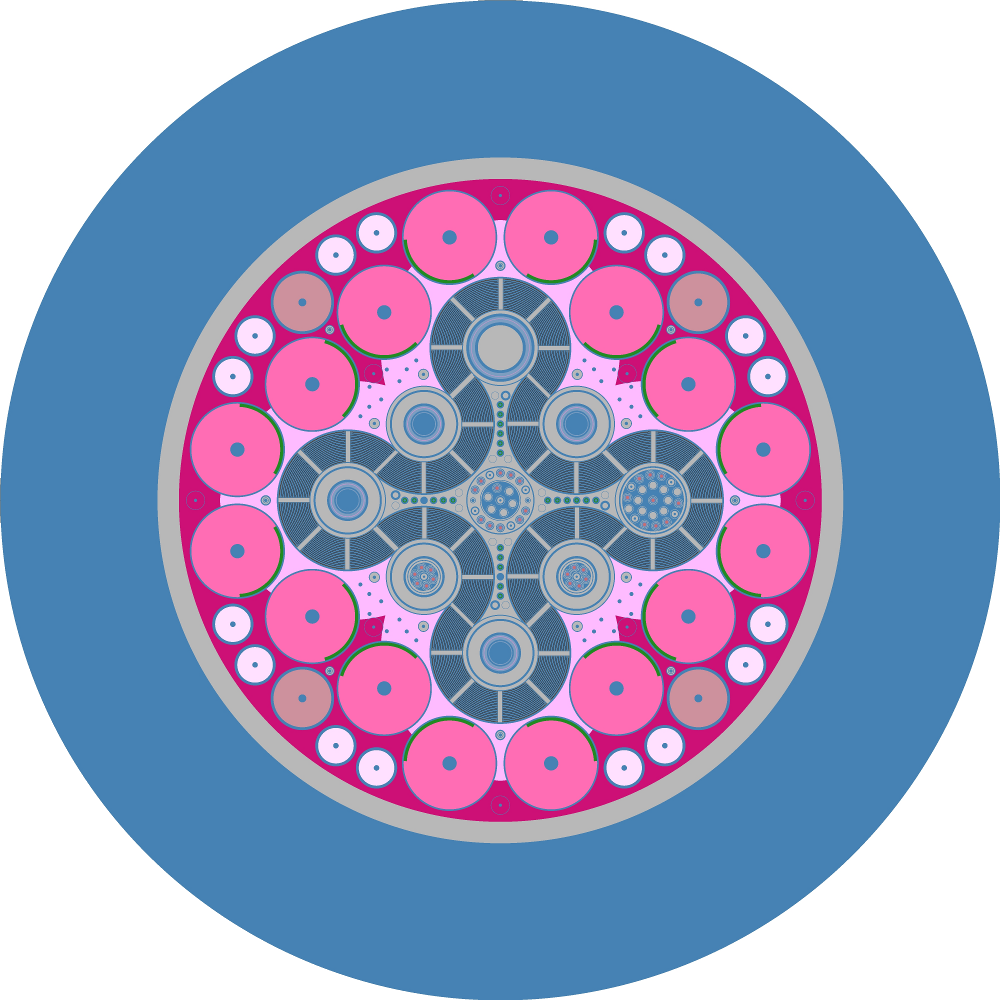
By default, when an instance of openmc.Plot is created, it indicates
that a 2D slice plot should be made. You can specify the origin of the plot
(Plot.origin), the width of the plot in each direction
(Plot.width), the number of pixels to use in each direction
(Plot.pixels), and the basis directions for the plot. For example, to
create a \(x\) - \(z\) plot centered at (5.0, 2.0, 3.0) with a width of
(50., 50.) and 400x400 pixels:
plot = openmc.Plot()
plot.basis = 'xz'
plot.origin = (5.0, 2.0, 3.0)
plot.width = (50., 50.)
plot.pixels = (400, 400)
The color of each pixel is determined by placing a particle at the center of
that pixel and using OpenMC’s internal find_cell routine (the same one used
for particle tracking during simulation) to determine the cell and material at
that location.
Note
In this example, pixels are 50/400=0.125 cm wide. Thus, this plot may miss any features smaller than 0.125 cm, since they could exist between pixel centers. More pixels can be used to resolve finer features but will result in larger files.
By default, a unique color will be assigned to each cell in the geometry. If you
want your plot to be colored by material instead, change the
Plot.color_by attribute:
plot.color_by = 'material'
If you don’t like the random colors assigned, you can also indicate that particular cells/materials should be given colors of your choosing:
plot.colors = {
    water: 'blue',
    clad: 'black'
}

# This is equivalent
plot.colors = {
    water: (0, 0, 255),
    clad: (0, 0, 0)
}
Note that colors can be given as RGB tuples or by a string indicating a valid SVG color.
When you’re done creating your openmc.Plot instances, you need to then
assign them to a openmc.Plots collection and export it to XML:
plots = openmc.Plots([plot1, plot2, plot3])
plots.export_to_xml()

# This is equivalent
plots = openmc.Plots()
plots.append(plot1)
plots += [plot2, plot3]
plots.export_to_xml()
To actually generate the plots, run the openmc.plot_geometry() function.
Alternatively, run the openmc executable with the --plot
command-line flag. When that has finished, you will have one or more .png
files. Alternatively, if you’re working within a Jupyter Notebook or QtConsole, you can use the
openmc.plot_inline() to run OpenMC in plotting mode and display the
resulting plot within the notebook.
9.2. Voxel Plots
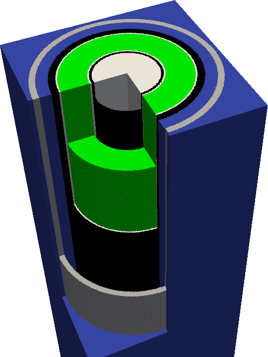
The openmc.Plot class can also be told to generate a 3D voxel plot
instead of a 2D slice plot. Simply change the Plot.type attribute to
‘voxel’. In this case, the Plot.width and Plot.pixels attributes
should be three items long, e.g.:
vox_plot = openmc.Plot()
vox_plot.type = 'voxel'
vox_plot.width = (100., 100., 50.)
vox_plot.pixels = (400, 400, 200)
The voxel plot data is written to an HDF5 file. The voxel file can subsequently be converted into a standard mesh format that can be viewed in ParaView, VisIt, etc. This typically will compress the size of the file significantly. The provided openmc-voxel-to-vtk script can convert the HDF5 voxel file to VTK formats. Once processed into a standard 3D file format, colors and masks can be defined using the stored ID numbers to better explore the geometry. The process for doing this will depend on the 3D viewer, but should be straightforward.
Note
3D voxel plotting can be very computer intensive for the viewing program (Visit, ParaView, etc.) if the number of voxels is large (>10 million or so). Thus if you want an accurate picture that renders smoothly, consider using only one voxel in a certain direction.
9.3. Projection Plots
The openmc.ProjectionPlot class presents an alternative method of
producing 3D visualizations of OpenMC geometries. It was developed to overcome
the primary shortcoming of voxel plots, that an enormous number of voxels must
be employed to capture detailed geometric features. Projection plots perform
volume rendering on material or cell volumes, with colors specified in the same
manner as slice plots. This is done using the native ray tracing capabilities
within OpenMC, so any geometry in which particles successfully run without
overlaps or leaks will work with projection plots.
One drawback of projection plots is that particle tracks cannot be overlaid on them at present. Moreover, checking for overlap regions is not currently possible with projection plots. The image heading this section can be created by adding the following code to the hexagonal lattice example packaged with OpenMC, before exporting to plots.xml.
r = 5
import numpy as np
for i in range(100):
    phi = 2 * np.pi * i/100
    thisp = openmc.ProjectionPlot(plot_id = 4 + i)
    thisp.filename = 'frame%s'%(str(i).zfill(3))
    thisp.look_at = [0, 0, 0]
    thisp.camera_position = [r * np.cos(phi), r * np.sin(phi), 6 * np.sin(phi)]
    thisp.pixels = [200, 200]
    thisp.color_by = 'material'
    thisp.colorize(geometry)
    thisp.set_transparent(geometry)
    thisp.xs[fuel] = 1.0
    thisp.xs[iron] = 1.0
    thisp.wireframe_domains = [fuel]
    thisp.wireframe_thickness = 2

    plot_file.append(thisp)
This generates a sequence of png files which can be joined to form a gif. Each
image specifies a different camera position using some simple periodic functions
to create a perfectly looped gif. ProjectionPlot.look_at defines where
the camera’s centerline should point at. ProjectionPlot.camera_position
similarly defines where the camera is situated in the universe level we seek to
plot. The other settings resemble those employed by openmc.Plot, with
the exception of the ProjectionPlot.set_transparent method and
ProjectionPlot.xs dictionary. These are used to control volume rendering
of material volumes. “xs” here stands for cross section, and it defines material
opacities in units of inverse centimeters. Setting this value to a large number
would make a material or cell opaque, and setting it to zero makes a material
transparent. Thus, the ProjectionPlot.set_transparent can be used to
make all materials in the geometry transparent. From there, individual material
or cell opacities can be tuned to produce the desired result.
Two camera projections are available when using these plots, perspective and orthographic. The default, perspective projection, is a cone of rays passing through each pixel which radiate from the camera position and span the field of view in the x and y positions. The horizontal field of view can be set with the :attr: ProjectionPlot.horizontal_field_of_view attribute, which is to be specified in units of degrees. The field of view only influences behavior in perspective projection mode.
In the orthographic projection, rays follow the same angle but originate from different points. The horizontal width of this plane of ray starting points may be set with the :attr: ProjectionPlot.orthographic_width element. If this element is nonzero, the orthographic projection is employed. Left to its default value of zero, the perspective projection is employed.
Lastly, projection plots come packaged with wireframe generation that can target
either all surface/cell/material boundaries in the geometry, or only wireframing
around specific regions. In the above example, we have set only the fuel region
from the hexagonal lattice example to have a wireframe drawn around it. This is
accomplished by setting the :attr: ProjectionPlot.wireframe_domains, which may
be set to either material IDs or cell IDs. The
ProjectionPlot.wireframe_thickness attribute sets the wireframe
thickness in units of pixels.
Note
When setting specific material or cell regions to have wireframes drawn around them, the plot must be colored by materials if wireframing around specific materials and similarly colored by cell instance if wireframing around specific cells.